Discrete Trait Analysis
Dowser implements recently developed phylogenetic tests to characterize B cell migration, differentiation, and isotype switching. These are “discrete” traits because their values are not continuous.
Discrete trait statistics
There are two main statistics implemented by Dowser to characterize the distribution of trait values at the tips of trees. These all derive from using a maximum parsimony algorithm to reconstruct trait values at the internal nodes of each tree. Then “switches” between discrete characters are quantified along the tree topologies.
- PS: Parsimony score, the total number of switches among all trait values.
- SP: Switch proportion, the proportion of switches from one trait to another.
The significance of each of these statistics is estimated using a permutation test, which randomizes trait values at the tree’s tips.
Full published details on these methods are available here
Caveats and interpretting results
Before using these tests, it’s important to understand how the test works and what potential biases can affect the results. These tests are detailed in full here.These tests summarize the distribution of trait values along trees. They don’t directly test for cellular migration and differentiation. As such, it’s important to understand potential caveats and explore alternative explanations.
What does a significant SP test mean? A significant SP test from tissue A to tissue B indicates that there is a greater proportion of switches from A to B along the trees than expected by random tip/trait relationships. This can be due to B cells preferentially migrating from tissue A to B, but there are other possibilities.
As explored in the original paper, a significant SP test from tissue A to B could be due to:
- Biased migration from A to B.
- Biased sampling, especially under-sampling tissue A.
- Significantly higher mutation rate over time in the cells in B than in A, placing it further down the tree.
- Extremely low rate of switching events (if no downsampling used, see below).
Usually option #1 is most biologically interesting, but it is important to consider the other options as well.
Setting up IgPhyML
All of the switch count statistics on this page require IgPhyML. IgPhyML needs to be compiled and the location of the executable needs to be passed to the findSwitches function. To set up IgPhyML, please visit the docs page. This is true even if IgPhyML is not used to build the trees. If you’re not using a Linux computer, your best option is likely to use the Immcantation Docker container.
Set up data structures and trees
This step proceeds as in tree building, but it is important to specify the column of the discrete trait you want to analyze in the formatClones step. In this example we are using simulated data from nose and lung biospies. However, this could be any discrete trait value such as cell types. Filtering out clones that contain only a single trait value type is not strictly necessary but can dramatically improve computing time.
library(dowser)

# load example AIRR tsv data
data(ExampleAirr)

# trait value of interest
trait="biopsy"

# Process example data using default settings
clones = formatClones(ExampleAirr,
    traits=trait, num_fields="duplicate_count", minseq=3)

# Column shows which biopsy the B cell was obtained from
print(table(ExampleAirr[[trait]]))
#Lung Nose
# 145  244

# Calculate number of tissues sampled in tree
tissue_types = unlist(lapply(clones$data, function(x)
  length(unique(x@data[[trait]]))))

# Filter to multi-type trees
clones = clones[tissue_types > 1,]

# Build trees using maximum likelihood (can use alternative builds if desired)
trees = getTrees(clones, build="pml")
Visualize maximum parsimony trait reconstruction
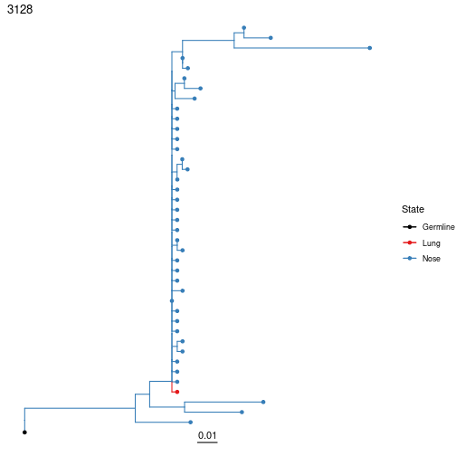
Sometimes it can be useful to visualize the predicted state of each internal node in the tree using maximum parsimony. In Dowser, this can be accomplished by modifying the getTrees call to specify the trait value of interest, and the location of the igphyml executable. The internal node states can be plotted using plotTrees with nodes=TRUE and tips specifying the trait value. Edges in the tree are colored by the predicted state of their descendant (lower) node.
# the location of the igphyml executable
# this is location in Docker image, will likely be different if you've set it up yourself
# note this is the location of the compiled executable file, not just the source folder
igphyml_location = "/usr/local/share/igphyml/src/igphyml"

# build trees as before, but use IgPhyML to reconstruct the states of internal
# nodes using maximum parsimony
trees = getTrees(clones, build="pml", trait=trait, igphyml=igphyml_location)

# show internal node (edge) predictions based on maximum parsimony
plotTrees(trees, tips=trait, nodes=TRUE, palette="Set1")[[1]]
Discrete trait analysis with fixed trees
Once we’ve set up the tree objects, we can calculate the switches along these trees using a maximum parsimony algorithm implemented in IgPhyML. We only need to perform this computationally intensive step once. All discrete trait tests use the resulting object. Note the IgPhyML location must be properly configured for your setup. Note also that your results may differ slightly from the ones shown below, due to the stochasticity of this test.
# the location of the igphyml executable
# this is location in Docker image, will likely be different if you've set it up yourself
# note this is the location of the compiled executable file, not just the source folder
igphyml_location = "/usr/local/share/igphyml/src/igphyml"

# calculate switches along trees compared to 100 random permutations
# this may take a while, and can be parallelized using nproc
switches = findSwitches(trees, permutations=100, trait=trait,
  igphyml=igphyml_location, fixtrees=TRUE)

# Perform PS test on switches
ps = testPS(switches$switches)
print(ps$means)
# A tibble: 1 x 6
#  RECON PERMUTE   PLT DELTA STAT   REPS
#  <dbl>   <dbl> <dbl> <dbl> <chr> <int>
#1     8     8.6   0.4  -0.6 PS      100


sp = testSP(switches$switches, alternative="greater")
print(sp$means)
# A tibble: 2 x 8
# Groups:   FROM [2]
#  FROM  TO    RECON PERMUTE   PGT  DELTA STAT   REPS
#  <chr> <chr> <dbl>   <dbl> <dbl>  <dbl> <chr> <int>
#1 Lung  Nose  0.131   0.323     1 -0.192 SP      100
#2 Nose  Lung  0.869   0.677     0  0.192 SP      100
PS test The object ps contains the results of the PS test. The means dataframe contains the test summary statistics, while the reps dataframe contains information from each repetition. RECON shows the number of switches across all trees, PERMUTE shows the mean number of switches across all permutations, and DELTA shows the mean difference between these two values. PLT is the P value that there are at least as many switches in the observed trees as in the permuted data. If PLT < 0.05, this indicates that there are signifcantly fewer switches among biopsies than expected by random tree/trait association. This indicates that sequences within the sample biopsies are more clustered together within the trees than expected. In this case, PLT is 0.4, so we can’t draw that conclusion.
SP test The object sp contains the results of the SP test. As with the PS test, the means dataframe contains summary statistics. The columns are largely the same as in the PS test, but the SP test is performed in a particular direction. In this case, we have an SP test from Lung to Nose and then from Nose to Lung. We can see that the SP value from Nose to Lung in our trees (RECON) is much higher than the mean SP statistic in our permuted trees (PERMUTE). DELTA is the mean difference between RECON and PERMUTE values, so a positive DELTA indicates greater SP values in observed trees than permuted trees. The p value in the PGT column (0) shows that the SP statistic from Nose to Lung is significant. This indicates that there are a greater proportion of switches from the Nose to the Lungs within these trees than expected from random tree/trait association. This is consistent with biased movement from Nose to Lungs in this dataset (but see Caveats and interpretting results section).
Accounting for uncertainty in tree topology
The previous analysis used fixed tree topologies, which will speed up calculations but does not account for uncertainty in tree topology. To account for this, be sure fixtrees=FALSE (the default option). For this option, the trees will be re-built for each permutation in the manner specified (same parameters as getTrees).
# calculate switches along bootstrap distribution of trees
# build using the 'pml' maximum likelihood option
# in a real analysis it's important to use at least 100 permutations
switches = findSwitches(trees, permutations=10, trait=trait,
  igphyml=igphyml_location, fixtrees=FALSE, build="pml")

sp = testSP(switches$switches, alternative="greater")
print(sp$means)
# A tibble: 2 x 8
# Groups:   FROM [2]
#  FROM  TO    RECON PERMUTE   PGT  DELTA STAT   REPS
#  <chr> <chr> <dbl>   <dbl> <dbl>  <dbl> <chr> <int>
#1 Lung  Nose  0.168   0.358   1   -0.190 SP       10
#2 Nose  Lung  0.832   0.642   0.1  0.190 SP       10
Within and between lineage permutations
In some cases it may be preferable to permute trait values among trees rather than within them. This will detect association between traits within a tree as well as directional relationships. In general it is harder to interpret. To perform this test, set permuteAll=TRUE.
sp = testSP(switches$switches, alternative="greater", permuteAll=TRUE)
print(sp$means)
# A tibble: 2 x 8
# Groups:   FROM [2]
#  FROM  TO    RECON PERMUTE   PGT   DELTA STAT   REPS
#  <chr> <chr> <dbl>   <dbl> <dbl>   <dbl> <chr> <int>
#1 Lung  Nose  0.168   0.241   0.6 -0.0736 SP       10
#2 Nose  Lung  0.832   0.759   0.4  0.0736 SP       10
Controlling false positive rate through downsampling
The SP test has been shown to have a high false positive rate if switching events are rare along very large trees (see paper). To reduce this effect, by default a downsampling algorithm in findSwitches will downsample all trees to have a maximum tip-to-switch ratio of 20. This ratio can be toggled by altering the tip_switch parameter. This feature can also be turned off by setting downsample=FALSE, but this is not recommended.
# Downsample each tree to a tip-to-switch ratio of 10 instead of 20
# this will reduce the false positive rate but also (likely) power
switches = findSwitches(trees, permutations=100, trait=trait,
  igphyml=igphyml_location, fixtrees=TRUE, tip_switch=10)

# didn't have much effect for this dataset
sp = testSP(switches$switches, alternative="greater")
print(sp$means)
# A tibble: 2 x 8
# Groups:   FROM [2]
#  FROM  TO    RECON PERMUTE   PGT  DELTA STAT   REPS
#  <chr> <chr> <dbl>   <dbl> <dbl>  <dbl> <chr> <int>
#1 Lung  Nose  0.168   0.358   1   -0.190 SP       10
#2 Nose  Lung  0.832   0.642   0.1  0.190 SP       10
Incorporating switching constraints
Some processes, like Ig isotype switching, can only happen in a particular direction. Using regular parsimony to reconstruct these processes will likely end up predicting impossible switches. Instead, it’s possible to contrain the maximum parsimony reconstruction to only happen in a particular direction. There are a couple of steps to do this.
- Create a vector with the states in the order they occur in.
- Create a model file with
makeModelFile. - Repeat maximum parsimony analyses with IgPhyML specifying the model file.
makeModelFile produces a physical file - you can open it with a text editor to inspect it. All runs of findSwitches create a model file, it’s just normally not seen by the user and by default contains no constraints.
# the location of the igphyml executable
# this is location in Docker image, will likely be different if you've set it up yourself
# note this is the location of the compiled executable file, not just the source folder
igphyml_location = "/usr/local/share/igphyml/src/igphyml"

# constant region column name
trait = "c_call"

# Vector of human isotypes in the proper order. Isotype switching
# can only go from left to right (e.g. IGHM to IGHA1). One exception
# is IGHD, which can switch to IGHM.
isotypes = c("IGHM","IGHD","IGHG3","IGHG1","IGHA1","IGHG2",
  "IGHG4","IGHE","IGHA2")

# Process example data using default settings with "c_call" as a trait value
clones = formatClones(ExampleAirr, traits=trait, minseq=3)

# Column shows which constant region associated with a BCR
print(table(ExampleAirr[[trait]]))
# IGHA1 IGHA2  IGHD IGHG1 IGHG2 IGHG3 IGHG4  IGHM
#    55    56    11    58    64    60    63    22

# Calculate number of istoypes sampled in each tree
isotype_counts = unlist(lapply(clones$data, function(x)
  length(unique(x@data[[trait]]))))

# make model file with irreversibility constraints
# Will prohibit switches from right to left in the "states" vector
# IGHD to IGHM switching listed as an exception, since this can occur
makeModelFile(file="isotype_model.txt", states=isotypes,
  constraints="irrev", exceptions=c("IGHD,IGHM"))

# Build trees and predict states at internal nodes using maximum parsimony
trees = getTrees(clones[isotype_counts > 1,], trait=trait, igphyml=igphyml_location,
  modelfile="isotype_model.txt")

# show internal node (edge) predictions based on maximum parsimony
plotTrees(trees, tips=trait, nodes=TRUE, palette="Paired", ambig="grey")[[1]]
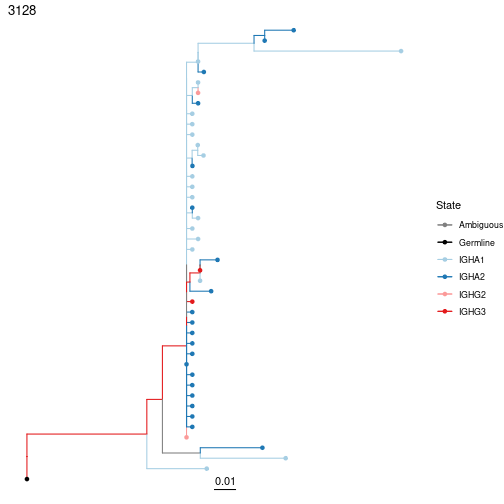
Performing the SP test is the same as before, just specify the model file created earlier using the modelfile option. Note that no switches occur in directions that are forbidden by our model. If you try this without specifying the model file, you’ll likely get many biologically impossible switches!
# Downsample each tree to a tip-to-switch ratio of 10 instead of 20
# this will reduce the false positive rate but also (likely) power
switches = findSwitches(trees, permutations=100, trait=trait,
  igphyml=igphyml_location, fixtrees=TRUE, tip_switch=10,
  modelfile="isotype_model.txt")

# didn't have much effect for this dataset
sp = testSP(switches$switches, alternative="greater")
print(sp$means,n=42)
# A tibble: 42 × 8
# Groups:   FROM [7]
#   FROM  TO      RECON PERMUTE   PGT     DELTA STAT   REPS
#   <chr> <chr>   <dbl>   <dbl> <dbl>     <dbl> <chr> <int>
# 1 IGHA1 IGHA2 0.0972  0.0994   0.56 -0.00219  SP      100
# 2 IGHA1 IGHD  0       0        1     0        SP      100
# 3 IGHA1 IGHG1 0       0        1     0        SP      100
# 4 IGHA1 IGHG2 0.00815 0.00833  0.58 -0.000184 SP      100
# 5 IGHA1 IGHG3 0       0        1     0        SP      100
# 6 IGHA1 IGHG4 0.00352 0.00409  0.59 -0.000575 SP      100
# 7 IGHA2 IGHA1 0       0        1     0        SP      100
# 8 IGHA2 IGHD  0       0        1     0        SP      100
# 9 IGHA2 IGHG1 0       0        1     0        SP      100
#10 IGHA2 IGHG2 0       0        1     0        SP      100
#11 IGHA2 IGHG3 0       0        1     0        SP      100
#12 IGHA2 IGHG4 0       0        1     0        SP      100
#13 IGHD  IGHA1 0       0        1     0        SP      100
#14 IGHD  IGHA2 0       0        1     0        SP      100
#15 IGHD  IGHG1 0.0144  0.0127   0.42  0.00173  SP      100
#16 IGHD  IGHG2 0.00926 0.00981  0.54 -0.000545 SP      100
#17 IGHD  IGHG3 0.0157  0.0113   0.3   0.00440  SP      100
#18 IGHD  IGHG4 0.00203 0.00271  0.58 -0.000681 SP      100
#19 IGHG1 IGHA1 0.00632 0.00757  0.59 -0.00126  SP      100
#20 IGHG1 IGHA2 0.00326 0.00419  0.51 -0.000932 SP      100
#21 IGHG1 IGHD  0       0        1     0        SP      100
#22 IGHG1 IGHG2 0.0417  0.0545   0.86 -0.0127   SP      100
#23 IGHG1 IGHG3 0       0        1     0        SP      100
#24 IGHG1 IGHG4 0.0451  0.0493   0.66 -0.00427  SP      100
#25 IGHG2 IGHA1 0       0        1     0        SP      100
#26 IGHG2 IGHA2 0.00542 0.00511  0.45  0.000316 SP      100
#27 IGHG2 IGHD  0       0        1     0        SP      100
#28 IGHG2 IGHG1 0       0        1     0        SP      100
#29 IGHG2 IGHG3 0       0        1     0        SP      100
#30 IGHG2 IGHG4 0.0715  0.0581   0.08  0.0133   SP      100
#31 IGHG3 IGHA1 0.0716  0.0600   0.16  0.0116   SP      100
#32 IGHG3 IGHA2 0.0508  0.0492   0.37  0.00154  SP      100
#33 IGHG3 IGHD  0       0        1     0        SP      100
#34 IGHG3 IGHG1 0.159   0.181    0.96 -0.0225   SP      100
#35 IGHG3 IGHG2 0.228   0.203    0.05  0.0250   SP      100
#36 IGHG3 IGHG4 0.161   0.175    0.8  -0.0137   SP      100
#37 IGHG4 IGHA1 0       0        1     0        SP      100
#38 IGHG4 IGHA2 0.00596 0.00437  0.27  0.00159  SP      100
#39 IGHG4 IGHD  0       0        1     0        SP      100
#40 IGHG4 IGHG1 0       0        1     0        SP      100
#41 IGHG4 IGHG2 0       0        1     0        SP      100
#42 IGHG4 IGHG3 0       0        1     0        SP      100
If you’re interested only in switches to a particular tissue or isotype, you can specify this using the to option in the testSP function. Here, we only look at the proportion of switches that go to IGHA2:
sp = testSP(switches$switches, alternative="greater", to="IGHA2")
print(sp$means)
# A tibble: 8 × 8
# Groups:   FROM [8]
#  FROM  TO     RECON PERMUTE   PGT    DELTA STAT   REPS
#  <chr> <chr>  <dbl>   <dbl> <dbl>    <dbl> <chr> <int>
#1 IGHA1 IGHA2 0.620   0.634   0.59 -0.0144  SP      100
#2 IGHD  IGHA2 0       0       1     0       SP      100
#3 IGHE  IGHA2 0       0       1     0       SP      100
#4 IGHG1 IGHA2 0.0116  0.0292  0.85 -0.0176  SP      100
#5 IGHG2 IGHA2 0.0371  0.0252  0.32  0.0119  SP      100
#6 IGHG3 IGHA2 0.297   0.283   0.45  0.0144  SP      100
#7 IGHG4 IGHA2 0.0346  0.0290  0.36  0.00563 SP      100
#8 IGHM  IGHA2 0       0       1     0       SP      100