Measurable evolution
Dowser implements recently developed phylogenetic tests to detect measurable B cell evolution from longitudinally sampled data.
Date randomization test
The goal of this test is to determine if a B cell lineage has a detectable relationship between mutation and time. If a lineage is accumulating new mutations over a sample interval, we expect a positive correlation between the divergence (sum of branch length to the most recent common ancestor, MRCA) and time elapsed.
Full published details on these methods is available here
Set up data structures and trees
This step proceeds as in tree building, but it is important to specify the column of the numeric time point values in the formatClones step. In this example we are using simulated data from timepoints 0, 7, and 14 days. Filtering out clones that contain only a single timepoint is not strictly necessary but can improve computing time.
Note it is critical that the clone object is formatted properly using formatClones with the trait option specified to the sample time. The sample time must be numeric.
library(dowser)

# load example AIRR tsv data
data(ExampleAirr)

# Process example data using default settings
clones = formatClones(ExampleAirr, traits="timepoint", minseq=3)

# Column shows timepoints in dataset
print(table(ExampleAirr$timepoint))
#0   7  14
#62 102 225

# Calculate number of tissues sampled in tree
timepoints = unlist(lapply(clones$data, function(x)
  length(unique(x@data$timepoint))))

# Filter to multi-type trees
clones = clones[timepoints > 1,]

# Build trees using maximum likelihood (can use alternative builds if desired)
trees = getTrees(clones, build="pml")
Perform date randomization test
Once trees have been built, perform the date randomization test using the function correlationTest. By default this test will use a clustered version of the date randomization test that corrects for issues like biased sampling of cell subpopulations, as well as types of sequencing error.
# correlation test with 10000 repetitions
test = correlationTest(trees, permutations=10000, time="timepoint")
print(test)

# A tibble: 6 × 12
#  clone_id data       locus  seqs trees      slope     p corre…¹ random…²  min_p
#     <dbl> <list>     <chr> <int> <list>     <dbl> <dbl>   <dbl>    <dbl>  <dbl>
#1     3128 <airrClon> N        40 <phylo> -0.00205 0.859  -0.173 -0.0257  0.0667
#2     3184 <airrClon> N        12 <phylo>  0.00111 0.497   0.649 -0.00429 0.5
#3     3140 <airrClon> N         9 <phylo>  0.00156 0.335   0.630 -0.00835 0.333
#4     3192 <airrClon> N         9 <phylo>  0.00739 0.498   0.956 -0.00306 0.5
#5     3115 <airrClon> N         6 <phylo>  0.00159 0.244   0.565  0.00236 0.25
#6     3139 <airrClon> N         6 <phylo>  0.00308 0.507   0.821  0.0112  0.5


# use uniform correlaion test (more sensitive, but higher false positive rate)
utest = correlationTest(trees, permutations=10000, time="timepoint", perm_type="uniform")
print(utest)

# A tibble: 6 × 12
#  clone_id data       locus  seqs trees      slope      p correlation random_c…¹
#     <dbl> <list>     <chr> <int> <list>     <dbl>  <dbl>       <dbl>      <dbl>
#1     3128 <airrClon> N        40 <phylo> -0.00205 0.856       -0.173   0.00146
#2     3184 <airrClon> N        12 <phylo>  0.00111 0.0768       0.649  -0.00223
#3     3140 <airrClon> N         9 <phylo>  0.00156 0.114        0.630   0.00205
#4     3192 <airrClon> N         9 <phylo>  0.00739 0.110        0.956   0.000223
#5     3115 <airrClon> N         6 <phylo>  0.00159 0.336        0.565   0.00409
#6     3139 <airrClon> N         6 <phylo>  0.00308 0.172        0.821   0.00431
The correlationTest function returns the same object that was provided as input, but with additional columns. The most important of which is the p value column. This gives the p value for the test that the observed correlation between divergence at time (correlation column) is greater than in trees with permuted time labels (random_correlation shows the mean of randomized correlations). The slope column shows the slope of the linear regression line between divergence and time, and represents the mean rate of evolution over time in the lineage. By default, permutations are performed using a clustered permutation procedure detailed in Hoehn et al. 2021. This adjusts for confounders like biased sampling at different timepoints and some forms of sequencing error. Uniform permutations, where the timepoint at each tip is permuted independently, can be used by setting perm_type="uniform". This may increase power for small datasets, but will likely increase the false positive rate.
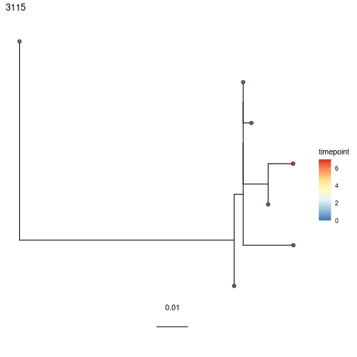
Plot trees
Plotting trees with time values on the tips is simple. Just specify the time column as the tips value in plotTrees. This is detailed in the Plotting Trees Vignette. There are many ways to customize these plots. Personally, I (Ken) typically use the following options for visualizing longitudinal data:
library(ggtree)

# order trees by p value
test = test[order(test$p),]

# Plot times on tree with lowest p value (not convincingly evolving)
plotTrees(test)[[1]] +
    geom_tippoint(aes(fill=timepoint), pch=21, size=2) +
    scale_fill_distiller(palette="RdYlBu")